ピリオドグラムにおけるバイアスとばらつき

この例では、ピリオドグラムにおけるバイアスとばらつきを減らす方法を示します。ウィンドウを使用すると、ピリオドグラムにおけるバイアスを減らすことができます。また、平均化機能のあるウィンドウを使用してばらつきを減らすことができます。

広義定常性自己回帰 (AR) 過程を使用して、ピリオドグラムにおけるバイアスとばらつきの影響を見ます。AR 過程は、その PSD が閉形式表現のため、扱いやすいモデルを提供します。次の形式の AR(2) モデルを作成します。

$y (n) - 0.75 y (n - 1) + 0.5 y (n - 2) = ε (n),$

ここで、 $ε (n)$ は、いくつかの指定分散を持つゼロ平均のホワイトノイズ列です。この例では、分散 1、サンプリング周期 1 と仮定します。上記の AR(2) 過程をシミュレートするには、全極 (IIR) フィルターを作成します。フィルターの振幅応答を表示します。

B2 = 1;
A2 = [1 -0.75 0.5];
freqz(B2,A2)

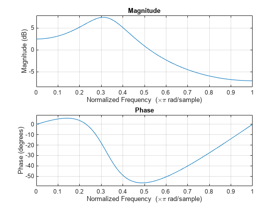
$Figure contains 2 axes objects. Axes object 1 with title Phase, xlabel Normalized Frequency (\times\pi rad/sample), ylabel Phase (degrees) contains an object of type line. Axes object 2 with title Magnitude, xlabel Normalized Frequency (\times\pi rad/sample), ylabel Magnitude (dB) contains an object of type line.$

この過程はバンドパスです。PSD のダイナミックレンジは約 14.5 dB で、これは次のコードで算出できます。

[H2,W2] = freqz(B2,A2);
dr2 = max(mag2db(abs(H2)))-min(mag2db(abs(H2)))

dr2 = 14.4982

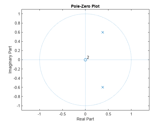
極の配置を調べることによって、この AR(2) 過程が安定であることがわかります。2 つの極は単位円の中にあります。

zplane(B2,A2)

Figure contains an axes object. The axes object with title Pole-Zero Plot, xlabel Real Part, ylabel Imaginary Part contains 4 objects of type line, text. One or more of the lines displays its values using only markers

次に、以下の式で表される AR(4) 過程を作成します。

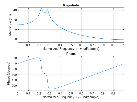
$y (n) - 2.7607 y (n - 1) + 3.8106 y (n - 2) - 2.6535 y (n - 3) + 0.9238 y (n - 4) = ε (n) .$

次のコードを使用して、この IIR システムの振幅応答を表示します。

B4 = 1;
A4 = [1 -2.7607 3.8106 -2.6535 0.9238];
freqz(B4,A4)

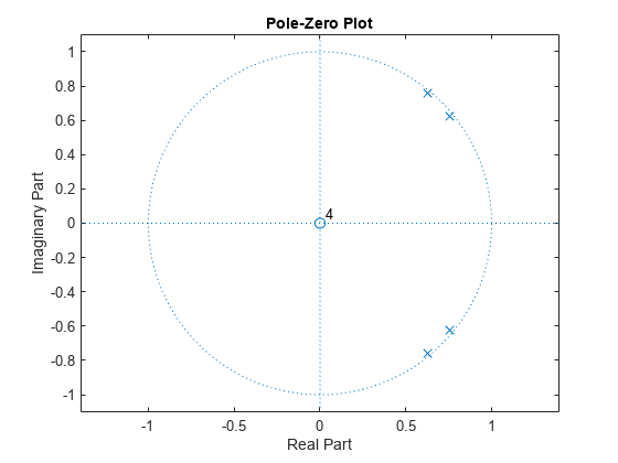
極の配置を調べることによって、この AR(4) 過程も安定であることがわかります。4 つの極は単位円の中にあります。

zplane(B4,A4)

この PSD のダイナミックレンジは約 65 dB で、AR(2) モデルよりはるかに大きな値です。

[H4,W4] = freqz(B4,A4);
dr4 = max(mag2db(abs(H4)))-min(mag2db(abs(H4)))

dr4 = 64.6343

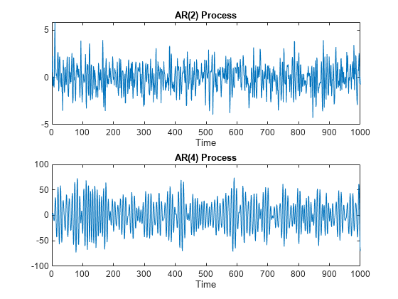
これらの AR(p) 過程からの実現をシミュレートするには、randn と filter を使用します。結果に再現性をもたせるために、乱数発生器を既定の設定にします。実現をプロットします。

rng default
x = randn(1e3,1);
y2 = filter(B2,A2,x);
y4 = filter(B4,A4,x);

subplot(2,1,1)
plot(y2)
title("AR(2) Process")
xlabel("Time")

subplot(2,1,2)
plot(y4)
title("AR(4) Process")
xlabel("Time")

Figure contains 2 axes objects. Axes object 1 with title AR(2) Process, xlabel Time contains an object of type line. Axes object 2 with title AR(4) Process, xlabel Time contains an object of type line.

AR(2) および AR(4) 実現のピリオドグラムを計算してプロットします。結果を実際の PSD と比較します。

subplot(2,1,1)
periodogram(y2)
hold on
plot(W2/pi,mag2db(abs(H2)/sqrt(pi)))
title("AR(2) PSD and Periodogram")
hold off

subplot(2,1,2)
periodogram(y4)
hold on
plot(W4/pi,mag2db(abs(H4)/sqrt(pi)))
title("AR(4) PSD and Periodogram")
text(0.6,10,"\downarrow Bias")
hold off

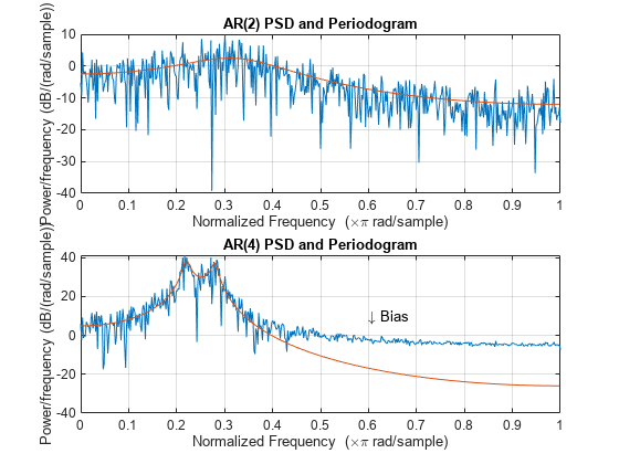
$Figure contains 2 axes objects. Axes object 1 with title AR(2) PSD and Periodogram, xlabel Normalized Frequency (\times\pi rad/sample), ylabel Power/frequency (dB/(rad/sample)) contains 2 objects of type line. Axes object 2 with title AR(4) PSD and Periodogram, xlabel Normalized Frequency (\times\pi rad/sample), ylabel Power/frequency (dB/(rad/sample)) contains 3 objects of type line, text.$

AR(2) 過程の場合、ピリオドグラム推定は真の PSD の形状に従いますが、かなりのばらつきを示します。これは、自由度が小さいことによるものです。ピリオドグラムにおける顕著な負の偏差 (dB) は、自由度 2 のカイ二乗確率変数の対数を取ることにより説明されます。

AR(4) 過程の場合、ピリオドグラムは低周波数では真の PSD の形状に従いますが、高周波数では真の PSD から逸脱しています。これはフェイェール核を伴う畳み込みの影響です。AR(2) 過程に比べて AR(4) 過程の大きなダイナミックレンジは、バイアスをより顕著にするものです。

AR(4) 過程内に示されたバイアスをテーパーまたはウィンドウを使用して緩和します。この例では、ピリオドグラムを求める前に、ハミングウィンドウを使用して AR(4) 実現にテーパーをかけます。

figure
periodogram(y4,hamming(length(y4)))
hold on
plot(W4/pi,mag2db(abs(H4)/sqrt(pi)))
title("AR(4) PSD and Periodogram with Hamming Window")
legend("Periodogram","AR(4) PSD")
hold off

Figure contains an axes object. The axes object with title AR(4) PSD and Periodogram with Hamming Window, xlabel Normalized Frequency ( times pi blank rad/sample), ylabel Power/frequency (dB/(rad/sample)) contains 2 objects of type line. These objects represent Periodogram, AR(4) PSD.

ここで、ピリオドグラム推定は、ナイキスト周波数範囲全体で真の AR(4) PSD に従っていることに注意してください。ピリオドグラム推定は引き続き自由度 2 しかもたないため、ウィンドウを使用してもピリオドグラムのばらつきは低減されません。しかし、ウィンドウを使用することでバイアスは解決します。

ノンパラメトリックスペクトル推定において自由度を増やしてピリオドグラムのばらつきを低減する 2 つの方法は、ウェルチのオーバーラップセグメント平均およびマルチテーパースペクトル推定です。

時間と半帯域幅との積として 3.5 を使用して、AR(4) 時系列のマルチテーパー推定を求めます。結果をプロットします。

NW = 3.5;

pmtm(y4,NW)
hold on
plot(W4/pi,mag2db(abs(H4)/sqrt(pi)))
legend("Multitaper Estimate","AR(4) PSD")
hold off

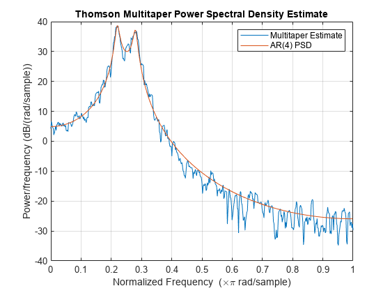
Figure contains an axes object. The axes object with title Thomson Multitaper Power Spectral Density Estimate, xlabel Normalized Frequency ( times pi blank rad/sample), ylabel Power/frequency (dB/(rad/sample)) contains 2 objects of type line. These objects represent Multitaper Estimate, AR(4) PSD.

マルチテーパー法は、ピリオドグラムよりばらつきが大幅に少ない PSD 推定を生成します。マルチテーパー法もウィンドウを使用しているので、ピリオドグラムのバイアスも解決していることがわかります。

参考

periodogram | pmtm