Preprocessing Raw Mass Spectrometry Data
This example shows how to improve the quality of raw mass spectrometry data. In particular, this example illustrates the typical steps for preprocessing protein surface-enhanced laser desorption/ionization-time of flight mass spectra (SELDI-TOF).
Loading the Data
Mass spectrometry data can be stored in different formats. If the data is stored in text files with two columns (the mass/charge (M/Z) ratios and the corresponding intensity values), you can use one of the following MATLAB® I/O functions: importdata, dlmread, or textscan. Alternatively, if the data is stored in JCAMP-DX formatted files, you can use the function jcampread. If the data is contained in a spreadsheet of an Excel® workbook, you can use the function xlsread.If the data is stored in mzXML formatted files, you can use the function mzxmlread, and finally, if the data is stored in SPC formatted files, you can use tgspcread.
This example uses spectrograms taken from one of the low-resolution ovarian cancer NCI/FDA data sets from the FDA-NCI Clinical Proteomics Program Databank. These spectra were generated using the WCX2 protein-binding chip, two with manual sample handling and two with a robotic sample dispenser/processor.
sample = importdata('mspec01.csv')
sample =

  struct with fields:

          data: [15154×2 double]
      textdata: {'M/Z'  'Intensity'}
    colheaders: {'M/Z'  'Intensity'}
The M/Z ratios are in the first column of the data field and the ion intensities are in the second.
MZ = sample.data(:,1);
Y  = sample.data(:,2);
For better manipulation of the data, you can load multiple spectrograms and concatenate them into a single matrix. Use the dlmread function to read comma separated value files. Note: This example assumes that the M/Z ratios are the same for the four files. For data sets with different M/Z ratios, use msresample to create a uniform M/Z vector.
files = {'mspec01.csv','mspec02.csv','mspec03.csv','mspec04.csv'};

for i = 1:4
    Y(:,i) = dlmread(files{i},',',1,1); % skips the first row (header)
end
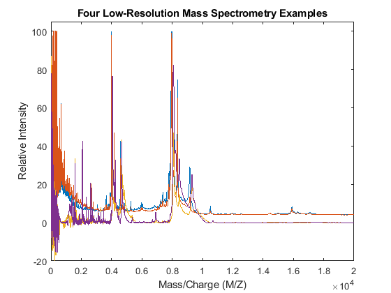
Use the plot command to inspect the loaded spectrograms.
plot(MZ,Y)
axis([0 20000 -20 105])
xlabel('Mass/Charge (M/Z)')
ylabel('Relative Intensity')
title('Four Low-Resolution Mass Spectrometry Examples')
Resampling the Spectra
Resampling mass spectrometry data has several advantages. It homogenizes the mass/charge (M/Z) vector, allowing you to compare different spectra under the same reference and at the same resolution. In high-resolution data sets, the large size of the files leads to computationally intensive algorithms. However, high-resolution spectra can be redundant. By resampling, you can decimate the signal into a more manageable M/Z vector, preserving the information content of the spectra. The msresample function allows you to select a new M/Z vector and also applies an antialias filter that prevents high-frequency noise from folding into lower frequencies.
Load a high-resolution spectrum taken from the high-resolution ovarian cancer NCI/FDA data set. For convenience, the spectrum is included in a MAT-formatted file.
load sample_hi_res
numel(MZ_hi_res)
ans =

      355760
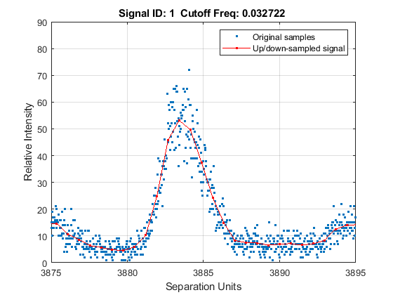
Down-sample the spectra to 10,000 M/Z points between 2,000 and 11,000. Use the SHOWPLOT property to create a customized plot that lets you follow and assess the quality of the preprocessing action.
[MZH,YH] = msresample(MZ_hi_res,Y_hi_res,10000,'RANGE',[2000 11000],'SHOWPLOT',true);

Zooming into a reduced region reveals the detail of the down-sampling procedure.
axis([3875 3895 0 90])
Baseline Correction
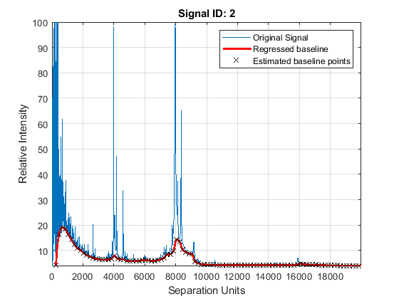
Mass spectrometry data usually show a varying baseline caused by the chemical noise in the matrix or by ion overloading. The msbackadj function estimates a low-frequency baseline, which is hidden among high-frequency noise and signal peaks. It then subtracts the baseline from the spectrogram.
Adjust the baseline of the set of spectrograms and show only the second one and its estimated background.
YB = msbackadj(MZ,Y,'WINDOWSIZE',500,'QUANTILE',0.20,'SHOWPLOT',2);
Spectral Alignment of Profiles
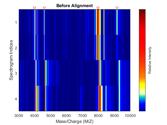
Miscalibration of the mass spectrometer leads to variations of the relationship between the observed M/Z vector and the true time-of-flight of the ions. Therefore, systematic shifts can appear in repeated experiments. When a known profile of peaks is expected in the spectrogram, you can use the function msalign to standardize the M/Z values.
To align the spectrograms, provide a set of M/Z values where reference peaks are expected to appear. You can also define a vector with relative weights that is used by the aligning algorithm to emphasize peaks with small area.
P = [3991.4 4598 7964 9160]; % M/Z location of reference peaks
W = [60 100 60 100];         % Weight for reference peaks
Display a heat map to observe the alignment of the spectra before and after applying the alignment algorithm.
msheatmap(MZ,YB,'MARKERS',P,'RANGE',[3000 10000])
title('Before Alignment')
Align the set of spectrograms to the reference peaks given.
YA = msalign(MZ,YB,P,'WEIGHTS',W);
msheatmap(MZ,YA,'MARKERS',P,'RANGE',[3000 10000])
title('After Alignment')
Normalization
In repeated experiments, it is common to find systematic differences in the total amount of desorbed and ionized proteins. The msnorm function implements several variations of typical normalization (or standardization) methods.
For example, one of many methods to standardize the values of the spectrograms is to rescale the maximum intensity of every signal to a specific value, for instance 100. It is also possible to ignore problematic regions; for example, in serum samples you might want to ignore the low-mass region (M/Z < 1000 Da.).
YN1 = msnorm(MZ,YA,'QUANTILE',1,'LIMITS',[1000 inf],'MAX',100);
figure
plot(MZ,YN1)
axis([0 10000 -20 150])
xlabel('Mass/Charge (M/Z)')
ylabel('Relative Intensity')
title('Normalized to the Maximum Peak')
The msnorm function can also standardize by using the area under the curve (AUC) and then rescale the spectrograms to have relative intensities below 100.
YN2 = msnorm(MZ,YA,'LIMITS',[1000 inf],'MAX',100);
figure
plot(MZ,YN2)
axis([0 10000 -20 150])
xlabel('Mass/Charge (M/Z)')
ylabel('Relative Intensity')
title('Normalized Using the Area Under the Curve (AUC)')
Peak Preserving Noise Reduction
Standardized spectra usually contain a mixture of noise and signal. Some applications require denoising of the spectrograms to improve the validity and precision of the observed mass/charge values of the peaks in the spectra. For the same reason, denoising also improves further peak detection algorithms. However, it is important to preserve the sharpness (or high-frequency components) of the peak as much as possible. For this, you can use Lowess smoothing (mslowess) and polynomial filters (mssgolay).
Smooth the spectrograms with a polynomial filter of second order.
YS = mssgolay(MZ,YN2,'SPAN',35,'SHOWPLOT',3);
Zooming into a reduced region reveals the detail of the smoothing algorithm.
axis([8000 9000 -1 8])
Peak Finding with Wavelets Denoising
A simple approach to find putative peaks is to look at the first derivative of the smoothed signal, then filer some of these locations to avoid small ion-intensity peaks.
P1 = mspeaks(MZ,YS,'DENOISING',false,'HEIGHTFILTER',2,'SHOWPLOT',1)
P1 =

  4×1 cell array

    {164×2 double}
    {171×2 double}
    {169×2 double}
    {147×2 double}
The mspeaks function can also estimate the noise using wavelets denoising. This method is generally more robust, because peak detection can be achieved directly over noisy spectra. The algorithm will adapt to varying noise conditions of the signal, and peaks can be resolved even if low resolution or oversegmentation exists.
P2 = mspeaks(MZ,YN2,'BASE',12,'MULTIPLIER',10,'HEIGHTFILTER',1,'SHOWPLOT',1)
P2 =

  4×1 cell array

    {322×2 double}
    {370×2 double}
    {324×2 double}
    {295×2 double}
Eliminate extra peaks in the low-mass region
P3 = cellfun( @(x) x(x(:,1)>1500,:),P2,'UNIFORM',false)
P3 =

  4×1 cell array

    {81×2 double}
    {93×2 double}
    {57×2 double}
    {53×2 double}
Binning: Peak Coalescing by Hierarchical Clustering
Peaks corresponding to similar compounds may still be reported with slight mass/charge differences or drifts. Assuming that the four spectrograms correspond to comparable biological/chemical samples, it might be useful to compare peaks from different spectra, which requires peak binning (a.k.a. peak coalescing). The crucial task in data binning is to create a common mass/charge reference vector (or bins). Ideally, bins should collect one peak from each signal and should avoid collecting multiple relevant peaks from the same signal into the same bin.
This example uses hierarchical clustering to calculate a common mass/charge reference vector. The approach is sufficient when using low-resolution spectra; however, for high-resolution spectra or for data sets with many spectrograms, the function mspalign provides other scalable methods to estimate a common mass/charge reference and perform data binning.
Put all the peaks into a single array and construct a vector with the spectrogram index for each peak.
allPeaks = cell2mat(P3);
numPeaks = cellfun(@(x) length(x),P3);
Sidx = accumarray(cumsum(numPeaks),1);
Sidx = cumsum(Sidx)-Sidx;
Create a custom distance function that penalizes clusters containing peaks from the same spectrogram, then perform hierarchical clustering.
distfun = @(x,y) (x(:,1)-y(:,1)).^2 + (x(:,2)==y(:,2))*10^6

tree = linkage(pdist([allPeaks(:,1),Sidx],distfun));
clusters = cluster(tree,'CUTOFF',75,'CRITERION','Distance');
distfun =

  function_handle with value:

    @(x,y)(x(:,1)-y(:,1)).^2+(x(:,2)==y(:,2))*10^6
The common mass/charge reference vector (CMZ) is found by calculating the centroids for each cluster.
CMZ = accumarray(clusters,prod(allPeaks,2))./accumarray(clusters,allPeaks(:,2));
Similarly, the maximum peak intensity of every cluster is also computed.
PR = accumarray(clusters,allPeaks(:,2),[],@max);

[CMZ,h] = sort(CMZ);
PR = PR(h);

figure
hold on
box on
plot([CMZ CMZ],[-10 100],'-k')
plot(MZ,YN2)
axis([7200 8500 -10 100])
xlabel('Mass/Charge (M/Z)')
ylabel('Relative Intensity')
title('Common Mass/Charge (M/Z) Locations found by Clustering')
Dynamic Programming Binning
The samplealign function allows you to use a dynamic programming algorithm to assign the observed peaks in each spectrogram to the common mass/charge reference vector (CMZ).
When simpler binning approaches are used, such as rounding the mass/charge values or using nearest neighbor quantization to the CMZ vector, the same peak from different spectra my be assigned to different bins due to the small drifts that still exist. To circumvent this problem, the bin size can be increased with the sacrifice of mass spectrometry peak resolution. By using dynamic programming binning, you preserve the resolution while minimizing the problem of assigning similar compounds from different spectrograms to different peak locations.
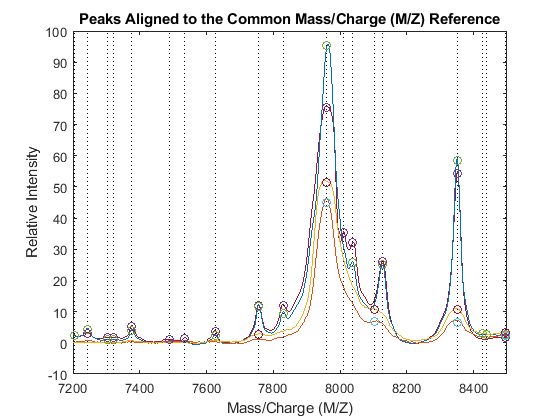
PA = nan(numel(CMZ),4);
for i = 1:4
    [j,k] = samplealign([CMZ PR],P3{i},'BAND',15,'WEIGHTS',[1 .1]);
    PA(j,i) = P3{i}(k,2);
end

figure
hold on
box on
plot([CMZ CMZ],[-10 100],':k')
plot(MZ,YN2)
plot(CMZ,PA,'o')
axis([7200 8500 -10 100])
xlabel('Mass/Charge (M/Z)')
ylabel('Relative Intensity')
title('Peaks Aligned to the Common Mass/Charge (M/Z) Reference')
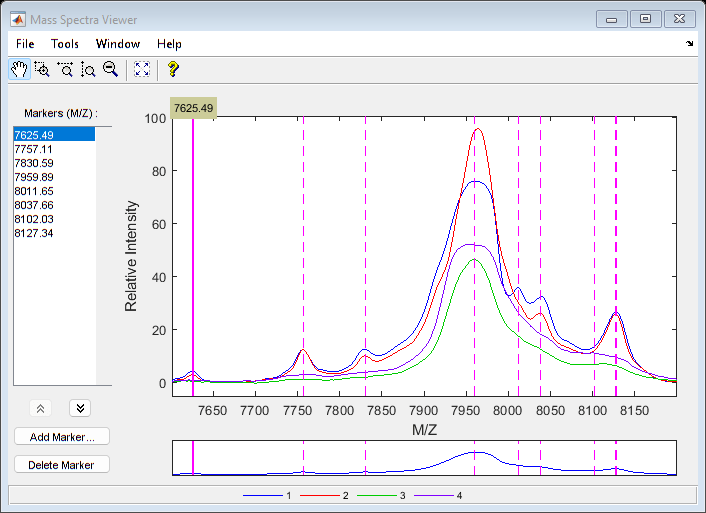
Use msviewer to inspect the preprocessed spectrograms on a given range (for example, between values 7600 and 8200).
r1 = 7600;
r2 = 8200;
range = MZ > r1 & MZ < r2;
rangeMarkers = CMZ(CMZ > r1 & CMZ < r2);

msviewer(MZ(range),YN2(range,:),'MARKERS',rangeMarkers,'GROUP',1:4)
See Also
mssgolay | msnorm | msalign | msheatmap | msbackadj | msresample | mspeaks | msviewer
Related Topics
You can also select a web site from the following list:
Americas
- América Latina (Español)
- Canada (English)
- United States (English)
Europe
- Belgium (English)
- Denmark (English)
- Deutschland (Deutsch)
- España (Español)
- Finland (English)
- France (Français)
- Ireland (English)
- Italia (Italiano)
- Luxembourg (English)
- Netherlands (English)
- Norway (English)
- Österreich (Deutsch)
- Portugal (English)
- Sweden (English)
- Switzerland
- United Kingdom (English)