Bootstrapping Phylogenetic Trees
This example shows how to generate bootstrap replicates of DNA sequences. The data generated by bootstrapping is used to estimate the confidence of the branches in a phylogenetic tree.
Introduction
Bootstrap, jackknife, and permutation tests are common tests used in phylogenetics to estimate the significance of the branches of a tree. This process can be very time consuming because of the large number of samples that have to be taken in order to have an accurate confidence estimate. The more times the data are sampled the better the analysis. A cluster of computers can shorten the time needed for this analysis by distributing the work to several machines and recombining the data.
Loading Sequence Data and Building the Original Tree
This example uses 12 pre-aligned sequences isolated from different hominidae species and stored in a FASTA-formatted file. A phylogenetic tree is constructed by using the UPGMA method with pairwise distances. More specifically, the seqpdist function computes the pairwise distances among the considered sequences and then the function seqlinkage builds the tree and returns the data in a phytree object. You can use the phytreeviewer function to visualize and explore the tree.
primates = fastaread('primatesaligned.fa');
num_seqs = length(primates)
num_seqs = 12
orig_primates_dist = seqpdist(primates);
orig_primates_tree =  seqlinkage(orig_primates_dist,'average',primates);
phytreeviewer(orig_primates_tree);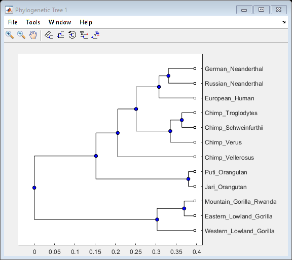
Making Bootstrap Replicates from the Data
A bootstrap replicate is a shuffled representation of the DNA sequence data. To make a bootstrap replicate of the primates data, bases are sampled randomly from the sequences with replacement and concatenated to make new sequences. The same number of bases as the original multiple alignment is used in this analysis, and then gaps are removed to force a new pairwise alignment. The function randsample samples the data with replacement. This function can also sample the data randomly without replacement to perform jackknife analysis. For this analysis, 100 bootstrap replicates for each sequence are created.
num_boots = 100;
seq_len = length(primates(1).Sequence);

boots = cell(num_boots,1);
for n = 1:num_boots
    reorder_index = randsample(seq_len,seq_len,true);
    for i = num_seqs:-1:1 %reverse order to preallocate memory
        bootseq(i).Header = primates(i).Header;
        bootseq(i).Sequence = strrep(primates(i).Sequence(reorder_index),'-','');
    end
    boots{n} = bootseq;
end
Computing the Distances Between Bootstraps and Phylogenetic Reconstruction
Determining the distances between DNA sequences for a large data set and building the phylogenetic trees can be time-consuming. Distributing these calculations over several machines/cores decreases the computation time. This example assumes that you have already started a MATLAB® pool with additional parallel resources. For information about setting up and selecting parallel configurations, see "Programming with User Configurations" in the Parallel Computing Toolbox™ documentation. If you do not have the Parallel Computing Toolbox™, the following PARFOR loop executes sequentially without any further modification.
fun = @(x) seqlinkage(x,'average',{primates.Header});
boot_trees = cell(num_boots,1);
parpool('local');
Starting parallel pool (parpool) using the 'local' profile ...
parfor (n = 1:num_boots)
    dist_tmp = seqpdist(boots{n});
    boot_trees{n} = fun(dist_tmp);
end
delete(gcp('nocreate'));
Counting the Branches with Similar Topology
The topology of every bootstrap tree is compared with that of the original tree. Any interior branch that gives the same partition of species is counted. Since branches may be ordered differently among different trees but still represent the same partition of species, it is necessary to get the canonical form for each subtree before comparison. The first step is to get the canonical subtrees of the original tree using the subtree and getcanonical methods from the Bioinformatics Toolbox™.
for i = num_seqs-1:-1:1  % for every branch, reverse order to preallocate
    branch_pointer = i + num_seqs;
    sub_tree = subtree(orig_primates_tree,branch_pointer);
    orig_pointers{i} = getcanonical(sub_tree);
    orig_species{i} = sort(get(sub_tree,'LeafNames'));
end
Now you can get the canonical subtrees for all the branches of every bootstrap tree.
for j = num_boots:-1:1
    for i = num_seqs-1:-1:1  % for every branch
        branch_ptr = i + num_seqs;
        sub_tree = subtree(boot_trees{j},branch_ptr);
        clusters_pointers{i,j} = getcanonical(sub_tree);
        clusters_species{i,j} = sort(get(sub_tree,'LeafNames'));
    end
end
For each subtree in the original tree, you can count how many times it appears within the bootstrap subtrees. To be considered as similar, they must have the same topology and span the same species.
count = zeros(num_seqs-1,1);
for i = 1 : num_seqs -1  % for every branch
    for j = 1 : num_boots * (num_seqs-1)
        if isequal(orig_pointers{i},clusters_pointers{j})
            if isequal(orig_species{i},clusters_species{j})
                count(i) = count(i) + 1;
            end
        end
    end
end

Pc = count ./ num_boots   % confidence probability (Pc)
Pc = 11×1

    1.0000
    1.0000
    0.9900
    0.9900
    0.5400
    0.5400
    1.0000
    0.4300
    0.3900
    0.3900
      ⋮
Visualizing the Confidence Values in the Original Tree
The confidence information associated with each branch node can be stored within the tree by annotating the node names. Thus, you can create a new tree, equivalent to the original primates tree, and annotate the branch names to include the confidence levels computed above. phytreeviewer displays this data in datatips when the mouse is hovered over the internal nodes of the tree.
[ptrs,dist,names] = get(orig_primates_tree,'POINTERS','DISTANCES','NODENAMES');

for i = 1:num_seqs -1  % for every branch
    branch_ptr = i + num_seqs;
    names{branch_ptr} = [names{branch_ptr} ', confidence: ' num2str(100*Pc(i)) ' %'];
end

tr = phytree(ptrs,dist,names)
Phylogenetic tree object with 12 leaves (11 branches)
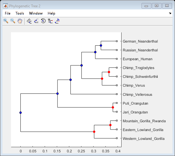
You can select the branch nodes with a confidence level greater than a given threshold, for example 0.9, and view these corresponding nodes in the Phylogenetic Tree app. You can also select these branch nodes interactively within the app.
high_conf_branch_ptr = find(Pc > 0.9) + num_seqs;
view(tr, high_conf_branch_ptr)
References
[1] Felsenstein, J., "Inferring Phylogenies", Sinaur Associates, Inc., 2004.
[2] Nei, M. and Kumar, S., "Molecular Evolution and Phylogenetics", Oxford University Press. Chapter 4, 2000.
You can also select a web site from the following list:
Americas
- América Latina (Español)
- Canada (English)
- United States (English)
Europe
- Belgium (English)
- Denmark (English)
- Deutschland (Deutsch)
- España (Español)
- Finland (English)
- France (Français)
- Ireland (English)
- Italia (Italiano)
- Luxembourg (English)
- Netherlands (English)
- Norway (English)
- Österreich (Deutsch)
- Portugal (English)
- Sweden (English)
- Switzerland
- United Kingdom (English)